The CSED Hackathon 2024
The CSED Hackathon tried to identify and correct the effect of stellar spots -literally spots on the surface of the star- in noisy transiting lightcurves of extrasolar planets. Exoplanets are planets orbiting other stars, like our own solar system planets orbit our sun. To date, we know over 4700 exoplanets in over 3400 solar systems (but this number changes daily so have a look here for a daily update).
When analysing these distant worlds, disentangling the effects of stellar activity and the non-linear noise of the instrument are the major data analysis challenges in the field and directly impacts our scientific measurements. Without correcting for brightness variabilities from the star and sensitivity variations of the instrument, we are not able to measure the radius of the planet correctly and, perhaps more importantly, the chemistry of their atmospheres. In the sections below we will explain some of the background on what an exoplanet observation consists of and how the problem of stellar spots comes into play.
The ESA ARIEL Space Mission
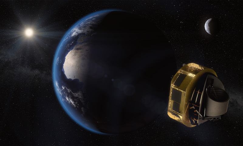
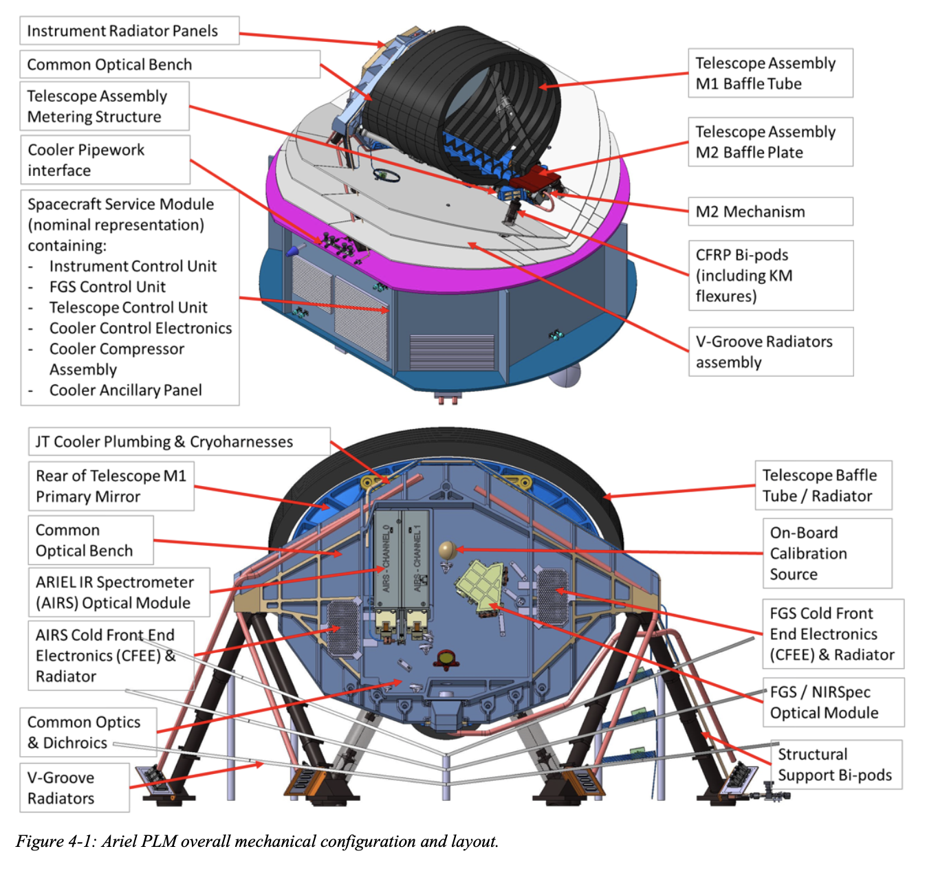
It’s probably best to first introduce the Ariel space mission for which the data used in this Hackathon (and the data challenge too!) was simulated. The Ariel mission is a European Space Agency (ESA) medium size mission (~500M Euros) to be launched to the second Lagrange point in 2029. The goal of the mission is to study the atmospheres and the chemistry of 1000 extrasolar planets (aka exoplanets) in our local galactic neighbourhood. By understanding their atmospheres, we can infer how these planets formed, what their natures are like and ultimately put our own solar system into context.
For loads more information on Ariel, here is the link to the website. There’s more information on exoplanets on the NASA exoplanet website or just google exoplanets. For a good podcast on exoplanets ExoCast.
What is a transit and a lightcurve?
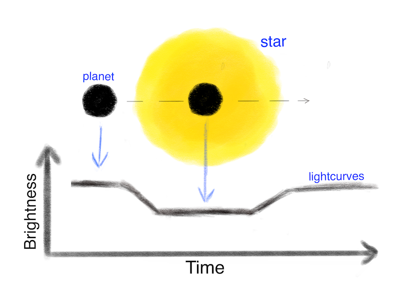
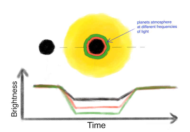
To start, what do we actually measure? Ariel will look at a class of exoplanets called ‘transiting exoplanets’. These are ~1% of the total exoplanets that pass in front of their host star in our line of sight. Essentially it’s the same as observing the transit of Venus but many lightyears away. We’ve drawn a sketch of what happens when the planet passes in front of the star (not to scale!). Some of the stellar light will be obscured by the planet and we observe a dip in the brightness of the star. This dip is directly proportional to the ratio of the areas of the planet and star. The bigger this ratio, the stronger that brightness dip will be. For a Jupiter size planet transiting a sun like star, we expect a 1% dip in light. For an Earth like planet, 0.001% around a sun-type star but around 1% when it orbits a much smaller M-star.
This dip in light over time is called a ‘lightcurve’. In the graphic below we show how this looks like.
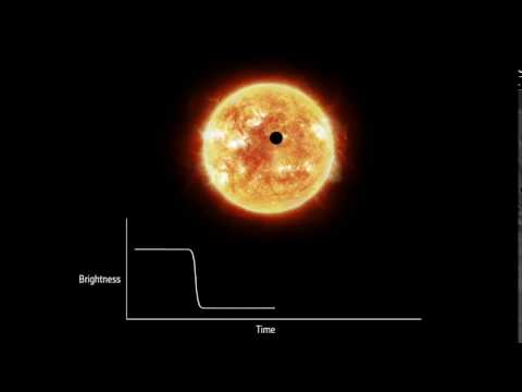
And a much more fancy (not hand drawn) animation of a transit (click to see):
Measuring the chemistry of an exoplanet
So we can measure the radius of the planet now by the dip in light of the star as the planet transits. How do we use that to study the chemistry, weather patterns and climate of the exoplanets’ atmospheres? Let’s assume the planet has an atmosphere. Some of the stellar light will filter through the thin atmospheric annulus surrounding the planet. We are typically speaking of 1 photon in 100,000 photons coming from the star passing through the annulus (also called the ‘terminator’). Next thing we need to know is that molecules absorb more or less light depending on the frequency/wavelength of the photon interacting with the molecule. This is also true for other absorbers such as clouds. Now if we look at a wavelength range of light where, say, water is a strong absorber, then we would expect fewer photons to reach us (as they get absorbed by the molecules in the atmosphere) than for wavelengths where no absorption happens (and the photon travels unimpeded through the atmosphere of the planet). Now if more photons get absorbed, that means fewer reach us, which in turn means that the lightcurve (the brightness dip) will look stronger/deeper to us. In effect, the planet will look ever so slightly bigger. By measuring this change in dip (aka ‘transit depth’) as function of wavelength/frequency of light, we can work out which molecules (or clouds) absorb photons in the atmosphere. With that, we can work out the chemistry, temperature, cloud coverage, wind speeds, climate and so much more of the planet. We’ve drawn another incredible diagram illustrating that:
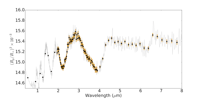
And when we translate the transit depth (i.e. the dip) into a spectrum then we get the plot below. What we see here is the depth of the lightcurve (Radius of Planet over Radius of Star squared… remember it’s the ratio of areas) on the y-axis and the walvength on the x-axis. This spectrum is a simulation of Ariel performances measuring a ‘famous’ hot-Jupiter HD209458b. The black points and orange bars are the measurements and errorbars overlaying the theoretical atmospheric model in grey.
HD209458b is a typical hot-Jupiter, a bit bigger than the Jupiter in our own Solar System and less massive, with an average temperature of ~1200C and a period (it’s year) of 3.5 days around its sun-like star. So quite hot and hostile…
What about star spots?
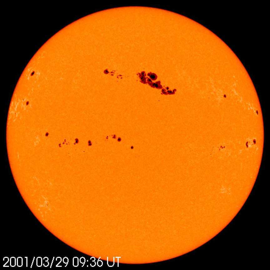
So why do we care about star spots then? And why is it such a big issue? Below is an image of spots on our own star, the sun. These are regions of lower brightness and temperature due to the emergence of strong magnetic field lines from the stellar surface. For sun-like stars, we have sun-spot cycles of about 11 years. Currently our own sun is at a solar minimum with very few spots as it is entering cycle 25 (counted since 1755). Other stars have different spot distributions and cycles, with stars smaller than the sun tending to be spottier (like teenagers) and large less spotty.
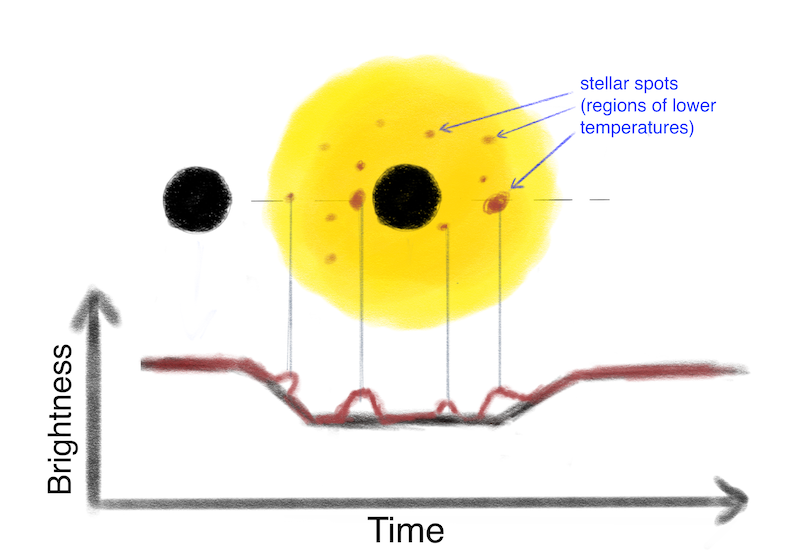
As you may easily imagine, if we now have a transit crossing a region of spots, it will mess up our otherwise pristine lightcurve with loads of bumps. The bumps make it difficult to measure the exact transit depth and without that, we have a very hard time to measure what the atmospheric spectrum is like and what it all means in terms of chemistry. Hence, detecting and ideally removing the spot contribution is paramount. Here’s another glorious diagram:
The main problem with removing spots is that in 99.9% of the cases, we do not know if the star has spots (and if we do know) where they are. So we cannot predict if a spot crossing event has happened. There is very little information for us to use to correct the spot signatures using astrophysical techniques. There are however a few helpful facts about spots.
As you will see in the data sets, the spot amplitudes are more pronounced in the shorter wavelengths (towards the visible light) than in the longer (infra-red). The more we go into the infra-red, the less spots we see. If we had a perfect instrument, we could simply take the difference between the visible and the infra-red to work out the spots. But there are two hindering factors: 1) The shape of the lightcurve changes with wavelength, in the short wavelengths it has a rounded bottom (due to stellar limb-darkening) whilst in the infra-red it looks more square (like in the diagrams); 2) Though there are fewer spots in the infra-red, we also have less star light which causes the noise on the lightcurve to increase significantly. So we have no spots but loads of noise in the infra-red, whilst we have low noise but loads of spots in the visible.
What about the instrument noise?
At the end of the light’s journey, it hits our telescopes and detectors. Analysing the atmospheres of extrasolar planets pushes us to the very limits of what contemporary technology can do. The Ariel space mission will be the first custom built space mission to do this work but even then, de-trending the instrument systematic noise (all non-Gaussian noise components) will be one of the main challenges. The noise sources of an instrument are varied and range from jitter noise (induced by the periodic wobble of a telescope as it tries to remain stable in free floating space) to quantum physics effects of its infra-red detectors. Space missions are intensely complicated and whilst every effort will be made to reduce the impact of instrument noise, some things cannot be avoided. The telescope will be cooled to -143 °C with the detectors even lower at -231 °C. This suppresses much of the noise but others remain.
In the sketch below, we illustrated two of the main effects that make analysis difficult: Detector persistence and non-Gaussian red-noise.
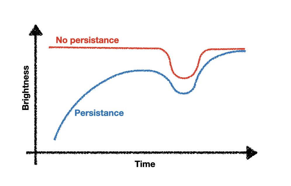
Persistence is one of the main and most common issues, it is characterised by a non-linear time-dependent change in sensitivity of the detector. This is obviously an issue if what you want to measure the precise change of flux hitting the detector as the exoplanet passes in front of its host-star. The sketch above shows an ideal observation over time in red, i.e. no time dependent trends. The blue curve is a sketch of typical persistance effects. Correcting for this trend is difficult as the trend varies with exoplanet observed (it is flux dependent), it varies with wavelength and it depends on what the previous observation has been. Here machine learning could help significantly to alleviate these effects.
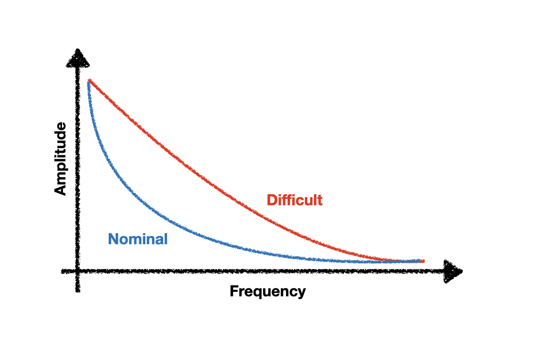
The other issue is the red-noise (or 1/f noise). This is determined by effects such as temperature fluctuations and vibrations, amongst others. Below we’ve sketched two fourier transforms of the noise. We have simulated two cases, the blue curve is the nominal case which has most noise concentrated in low-frequency modes. This is ideal as lower frequencies tend to be easier to track and de-trend. Modes that are of the order of the exoplanet transit time (1-2 hours) are the hardest as they can mimic an exoplanet transit event or worse, overlay the transit and corrupt the transit depth measurement (red curve). We’ll be simulating a mix of nominal and worst case scenarios for this hackathon.