The Science

This data challenge focuses on inverse modelling of atmospheric spectra of extrasolar planets (planets around other stars). Today we know of over 5000 planets outside our own solar system (this number changes daily so have a look here for a daily update). Extrasolar planets (aka exoplanets) range from Earth-like (such as the Trappist 1 system) to ultra-hot and inflated hot-Jupiters and everything in between. Though we have learned a lot about planet formation and the staggering diversity of worlds in our Milky Way, we are still very much at the beginning of being able to put our own solar system into the galactic context. In order to change this, the European Space Agency (in collaboration with NASA and JAXA) is building the Ariel Space Mission aiming to study the atmospheres of 1000 near by planets in detail and scheduled to be launched in 2029.

One of the main bottlenecks of this planet-characterisation work is the complexity of the planetary models. In order to make sense of what we observe, we need to model the complex processes happening in the atmospheres of those very exotic worlds, which involve complex chemistries, clouds and dynamics. The challenge is huge, we can barely do this for our own planet that we know so well, imagine the difficulty of trying to work out the nature of an unknown planet 10’s or 100’s of lightyears away. In addition, these atmospheric forward models require significant computing resources and are typically too slow to be used in a classic fitting/sampling setup using e.g. Markov Chain Monte Carlo or Nested Sampling.

This challenge will focus on developing inverse modelling methods that can map the observed atmospheric signatures to planetary characteristics (e.g. amount of water in the atmosphere, temperatures, clouds, etc).

We will provide a set of simulated atmospheric spectra, their corresponding ground-truth models and fitted Bayesian posterior distribtutions. To fit our data, we use the Nested Sampling MultiNest algorithm. The data set was generated with Alfnoor, which combines the open source TauREx 3 atmospheric modelling suite with the official Ariel instrument simulator ArielRad to produce large-scale simulations of atmospheres.

As part of this data challenge, we are providing walk-through jupiter notebooks on how the TauREx 3 code can be used to generate the data and how the data is fitted (we also call this ‘retrieval’) using Nested Sampling.

This permanent repository contains the Ariel Big Challenge (ABC) Database with Level 1 and 2 data, as well as various supporting ressources. In particular, it contains the “How to Use” Tutorial, which demonstrates how to load and explore the database. It also includes the “Taurex tutorial” with a small presentation on how to use the codes and two Jupyter notebooks. The notebook “TP_forward” describes the data generation and the notebook “TP_retrieval” describes the data fitting process.

Below, we run you through a high-level overview of the science.

We have also written a paper on the structure and content of the training data set. We strongly encourage you to have a look as it may help you design your solutions. The paper can be found here

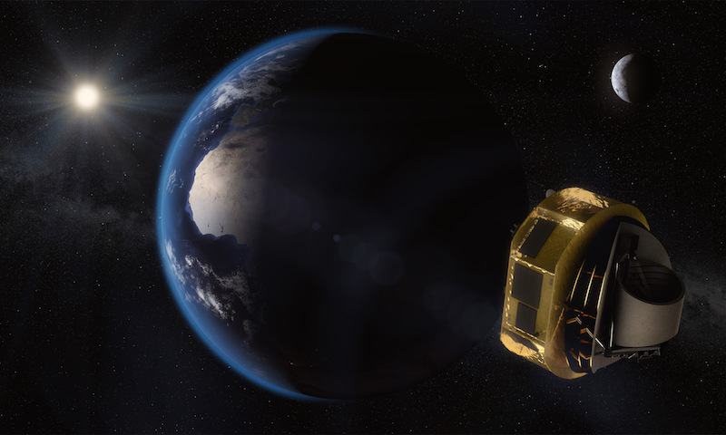
The ARIEL Space mission

It’s probably best to first introduce the Ariel space mission for which the data used in this challenge was simulated. The Ariel mission is a European Space Agency (ESA) medium size mission (~500M Euros) to be launched in 2029 to the second Lagrange point. The goal of the mission is to study the atmospheres and the chemistry of 1000 extrasolar planets in our local galactic neighbourhood. By understanding their atmospheres, we can infer how these planets formed, what their natures are like and ultimately put our own solar system into context.

For more information on Ariel, here is the link to the website and here is the Ariel Reference Redbook. There’s more information on exoplanets on the NASA exoplanet website or just google exoplanets. For a good podcast on exoplanets ExoCast.

What is a transit and a lightcurve?

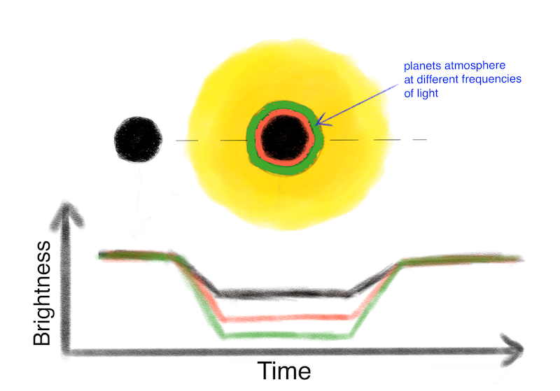
To start with, what do we actually measure? Ariel will look at a class of exoplanets called ‘transiting exoplanets’. These are exoplanets that pass in front of their host star in our line of sight, and they only represent about ~1% of the total exoplanet population. Essentially it’s the same as observing the transit of Venus but many lightyears away. Due to the large distances, we cannot resolve the planet itself, so we analyse the variations of light coming from the star. We’ve drawn a sketch of what happens when the planet passes in front of the star (not to scale!). Some of the stellar light will be obscured by the planet and we observe a dip in the brightness of the star. This dip is directly proportional to the ratio of the areas of the planet and star. The bigger this ratio, the stronger that brightness dip will be. For a Jupiter size planet transiting a star like our sun, we expect a 1% dip in the light we receive from the star when the transit happens. For an Earth like planet around a sun-type star, this is only 0.001%, but if the star is smaller like with M-star, it can be around 1%.

This dip in light over time is called a ‘lightcurve’. In the graphic below we show how this looks like.

Measuring the chemistry of an exoplanet

We can measure the radius of the planet via the dip its transit create on the light of the star. How do we use that to study the chemistry, weather patterns and climate of the exoplanets’ atmospheres? Let’s assume the planet has an atmosphere. Some of the stellar light will filter through the thin atmospheric annulus surrounding the planet. We are typically speaking of 1 photon in 100,000 photons coming from the star passing through the annulus (also called the ‘terminator’). In the illustration below, we show the planetary atmosphere as blue circles through which the stellar photons pass on their way to us, the observer.

Depending on the molecules present in the atmosphere, different colors of light (or wavelengths) will be absorbed or re-emitted by these molecules. In other words, the atmosphere’s chemistry will leave a characteristic fingerprint on the light that reaches us.
This is also true for other absorbers such as clouds or aerosols. Now if we look at a wavelength range of light where, say, water is a strong absorber, then we would expect fewer photons to reach us (as they get absorbed by the molecules in the atmosphere) than for wavelengths where no absorption happens (and the photon travels unimpeded through the atmosphere of the planet). Now if more photons get absorbed, that means fewer reach us, which in turn means that the lightcurve (the brightness dip) will look stronger/deeper to us. In effect, the planet will look ever so slightly bigger. By measuring this change in the dips (aka ‘transit depth’) as function of wavelength/frequency of light, we can work out which molecules (or clouds) absorb photons in the atmosphere. With that, we can understand the chemistry, temperature, cloud coverage, wind speeds, climate and so much more of the planet. The change in transit depth is only of the order or 0.001% of the light we receive from the star, so this is a very difficult observation. Below is a little hand-drawn illustration of the impact of a more opaque atmosphere on the transit depth for a given wavelength (green is more opague than red).

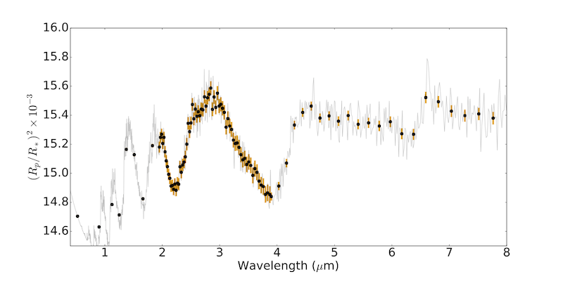
We can translate the transit depth (i.e. the dip) into a spectrum and we obtain the plot below. What we see here is the depth of the lightcurve (Radius of Planet over Radius of Star squared… remember it’s the ratio of surface area of the star and area occulted by the planet) on the y-axis and the wavelength (typically in micrometers) on the x-axis. This spectrum is a simulation of Ariel performances measuring a well-studied hot-Jupiter HD-209458 b. The black points and orange bars are the measurements and errorbars overlaying the theoretical atmospheric model in grey.

HD209458b is a typical hot-Jupiter, a bit bigger than Jupiter and less massive, with an average temperature of ~1200C and a period (it’s year) of 3.5 days around its sun-like star. So quite hot and hostile…

Interpreting the atmospheric spectrum

The usual method to interpret the atmospheric spectra of exoplanets is to ‘fit’ radiative transfer models to the spectrum. We typically use Bayesian inverse modelling. Let’s take the very famour super-Earth K2-18b as an example. K2-18b orbtis its red-dwarf star 124 lightyears from us and is roughly 8.6 Earth-masses and 2.6 Earth-radii big with an average temperature close to the freezing point of water (ca. 265 Kelvin). The planet’s spectrum was observed by the Hubble Space Telescope and can be seen below (black dots and errobars)

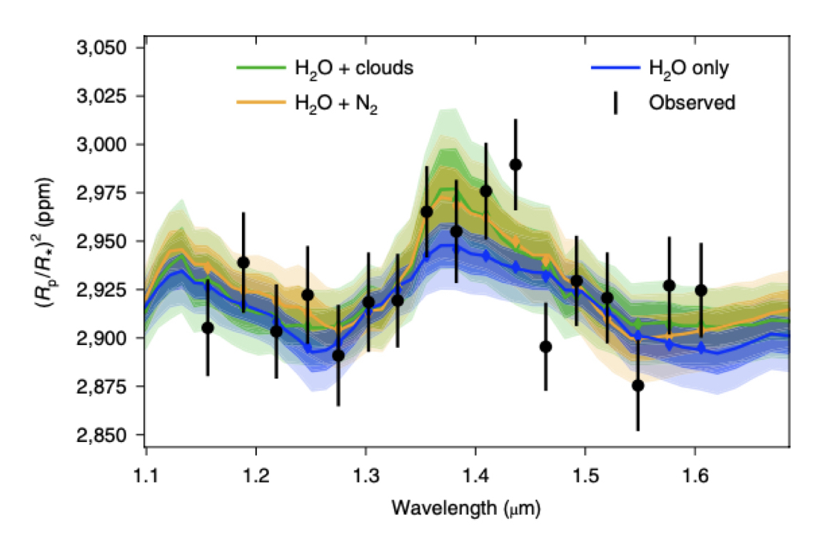
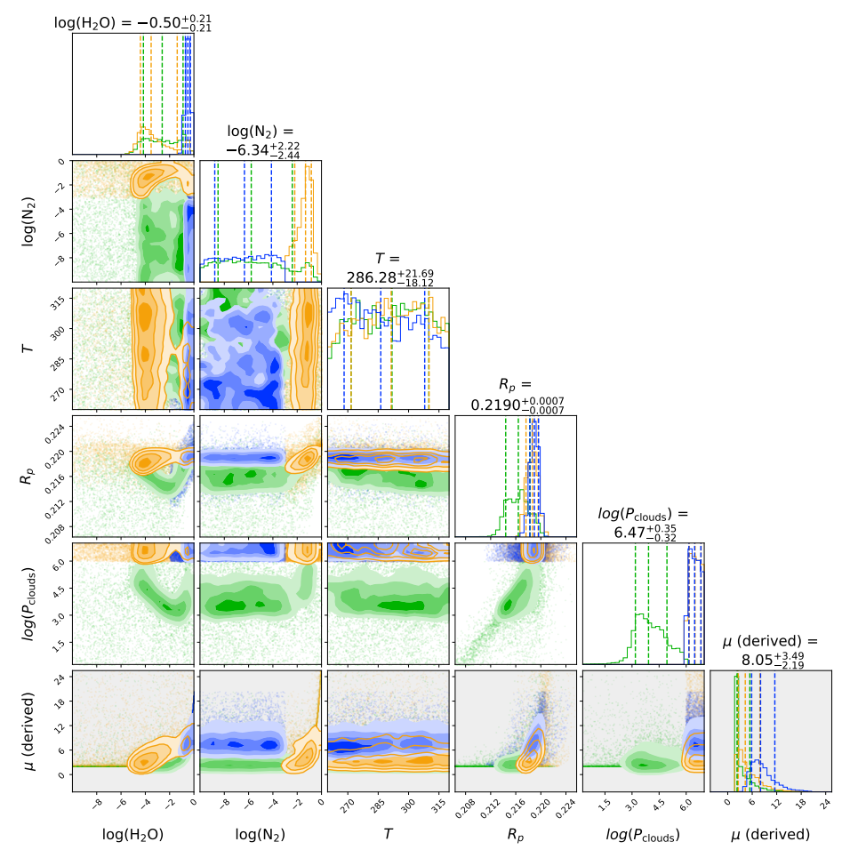
The different coloured models overplotted were generated by the TauREx 3 code (see here for the paper). You can see immediately that different atmospheric models with different assumptions fit similarly well. The Bayesian posterior distribution is shown below where it is clear that the atmospheric model parameters are all strongly correlated. In other words, our observations are too uncertain to constrain our atmospheric model precisely. In this case, the model contained the abundances of water (H₂O), nitrogen (N₂) and other planet parameters such as temperature (T), planet surface radius (R_P) and cloud top-pressure (i.e. height of the clouds in the atmosphere, P_clouds)

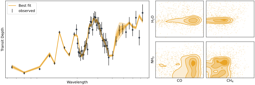
The Hubble Space Telescope was never designed to study extrasolar planet atmospheres and only allows us to study a small wavelength range. This is the reason why the Ariel mission concept was born and Ariel will be custom built and able to observe a far wider wavelength range, which will in-turn allow us to break many model degeneracies. Below is simulation of Ariel data and on the right the retrieved conditional posterior distributions of three forward model parameters. As you can see, even for Ariel, these posterior distributions are not trivial!

In this challenge, we ask you to come up with a faster method to solve the inverse problem. For this, we provided you with ~20k atmospheric models and simulated observations and ~5k posterior distributions (sampled using MultiNest). We provide a a baseline solution and description for you to get started here. We also provide a detailed description of the data and upload format in our documentation tab.

And finally, we wish you Good luck!