Documentation

We will be evaluating each submission on two metrics.
1. Posterior Scores - the similarities of participants’ set of 7 empirical univariate distributions to our ground truth, and
2. Spectral Score - the similarities between the submission and the ground truth in terms of the best-fit atmospheric spectra.

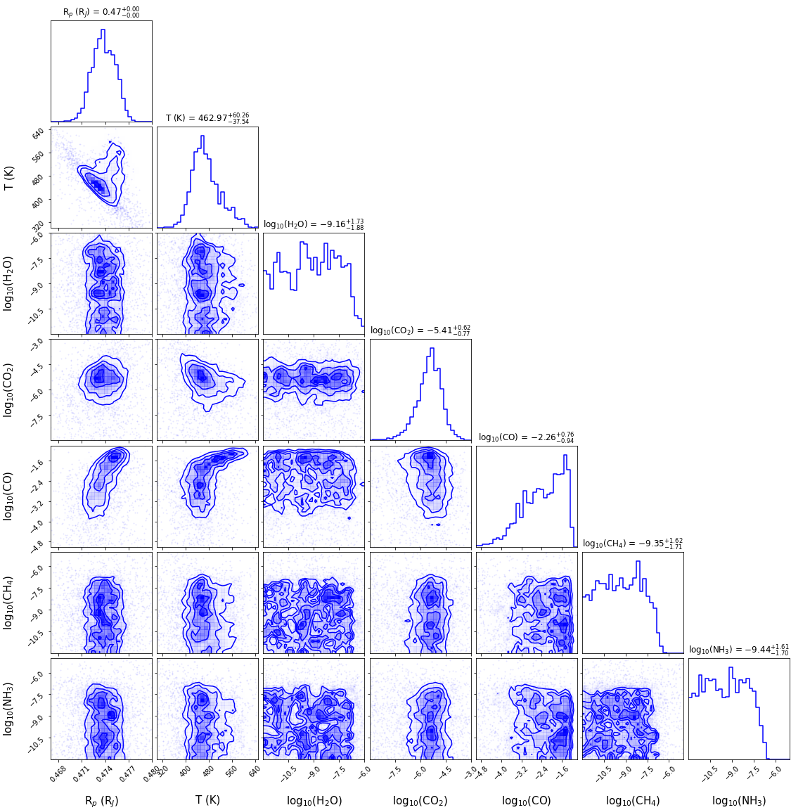
Conceptually, the two metrics complement each other and aim to reproduce the entirety of the corner plot below. The former ensures the submissions match each univariate conditional distribution (diagonal elements) produced from the sampling procedure. The second one enforces the laws of physics, or more accurately, the interaction (covariance) between different targets (the boxes under the diagonal). The ideal solution will be able to recognize the physical correlations between targets and produce distributions that comply with the Bayesian principle.

The image below shows a visual representation of the conditional distribution:

We will be using 2 Sample Kolmogorov–Smirnov test (K-S test) to test the posterior score case. The K-S test is commonly used to determine whether two given samples are originated from the same underlying continuous distribution. We implemented the K-S test using scipy.stats.ks_2samp and have modified the output so that it is bounded between 0 and 1000, with 1000 being the most similar.

As for the spectral score, we will be comparing the “median” in spectral space (a spectrum composed of the median value in each wavelength bin), and their uncertainty bounds (IQR value of each wavelength bin) against those coming from Bayesian Nested Sampling. Their differences are quantified using an inverse Huber loss. The spectral score will be a linear combination of the difference between bounds and difference between median spectra. The maximum score is again set to 1000, with 0 being the lowest and the least similar.

The final score is computed using the following formula:
$$\begin{equation} \text{final} = 0.2 \times \text{Score}_{Spectral} + 0.8 \times \text{Score}_{Posterior} \end{equation}$$
The final score is a weighted sum of the spectral_loss and posterior_loss, it has a minimum score of 0 and a maximum score of 1000.

To help you with the model evaluation, we have included the exact metric we used for the challenge here.